from subprocess import check_output print(check_output(["ls", "../input"]).decode("utf8")) #check the files available in the directory
sample_submission.csv
test.csv
train.csv
1
2
3
4
5
6
#Now let's import and put the train and test datasets in pandas dataframe
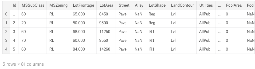
train = pd.read_csv('../input/train.csv') test = pd.read_csv('../input/test.csv') ##display the first five rows of the train dataset. train.head(5)
1
2
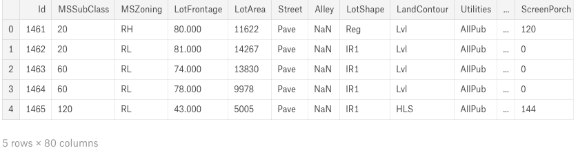
##display the first five rows of the test dataset.
test.head(5)
1
2
3
4
5
6
7
8
9
10
11
12
13
14
15
#check the numbers of samples and features
print("The train data size before dropping Id feature is : {} ".format(train.shape))
print("The test data size before dropping Id feature is : {} ".format(test.shape))

#Save the 'Id' column
train_ID = train['Id']
test_ID = test['Id']

#Now drop the  'Id' colum since it's unnecessary for  the prediction process.
train.drop("Id", axis = 1, inplace = True)
test.drop("Id", axis = 1, inplace = True)

#check again the data size after dropping the 'Id' variable
print("\nThe train data size after dropping Id feature is : {} ".format(train.shape))
print("The test data size after dropping Id feature is : {} ".format(test.shape))
1
2
3
4
5
6
>The train data size before dropping Id feature is : (1460, 81)
>The test data size before dropping Id feature is : (1459, 80)
>
>The train data size after dropping Id feature is : (1460, 80)
>The test data size after dropping Id feature is : (1459, 79)
>
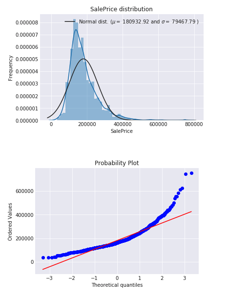
# Get the fitted parameters used by the function (mu, sigma) = norm.fit(train['SalePrice']) print( '\n mu = {:.2f} and sigma = {:.2f}\n'.format(mu, sigma))
#Now plot the distribution plt.legend(['Normal dist. ($\mu=$ {:.2f} and $\sigma=$ {:.2f} )'.format(mu, sigma)], loc='best') plt.ylabel('Frequency') plt.title('SalePrice distribution')
#Get also the QQ-plot fig = plt.figure() res = stats.probplot(train['SalePrice'], plot=plt) plt.show()
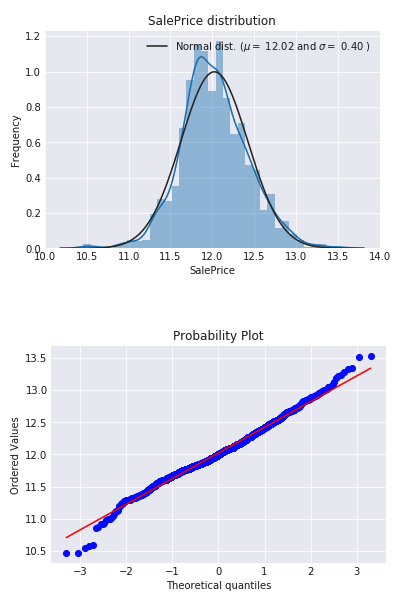
#We use the numpy fuction log1p which applies log(1+x) to all elements of the column train["SalePrice"] = np.log1p(train["SalePrice"])
#Check the new distribution sns.distplot(train['SalePrice'] , fit=norm);
# Get the fitted parameters used by the function (mu, sigma) = norm.fit(train['SalePrice']) print( '\n mu = {:.2f} and sigma = {:.2f}\n'.format(mu, sigma))
#Now plot the distribution plt.legend(['Normal dist. ($\mu=$ {:.2f} and $\sigma=$ {:.2f} )'.format(mu, sigma)], loc='best') plt.ylabel('Frequency') plt.title('SalePrice distribution')
#Get also the QQ-plot fig = plt.figure() res = stats.probplot(train['SalePrice'], plot=plt) plt.show()
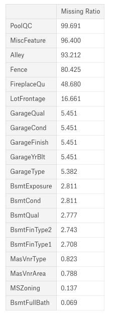
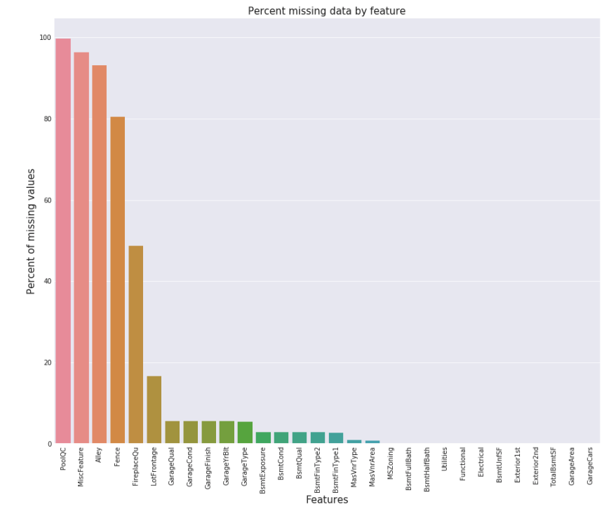
f, ax = plt.subplots(figsize=(15, 12)) plt.xticks(rotation='90') sns.barplot(x=all_data_na.index, y=all_data_na) plt.xlabel('Features', fontsize=15) plt.ylabel('Percent of missing values', fontsize=15) plt.title('Percent missing data by feature', fontsize=15)
1 2
>Text(0.5,1,'Percent missing data by feature') >
数据关联
1 2 3 4
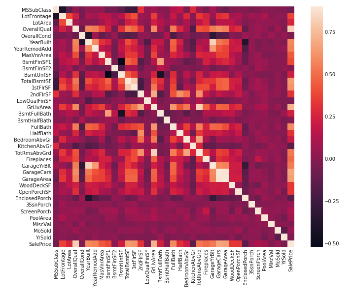
#Correlation map to see how features are correlated with SalePrice corrmat = train.corr() plt.subplots(figsize=(12,9)) sns.heatmap(corrmat, vmax=0.9, square=True)
输入缺失值
根据不同特征的不同情况对缺失值进行填充。
对于离散值且数据说明里有 NA 选项,则将缺失值补为None。
PoolQC : 数据描述说 NA 表示 “没有泳池”。这是有意义的,因为有大量的缺失数据,这表明大多数的房子都没有游泳池。
#Group by neighborhood and fill in missing value by the median LotFrontage of all the neighborhood all_data["LotFrontage"] = all_data.groupby("Neighborhood")["LotFrontage"].transform( lambda x: x.fillna(x.median()))
对于连续值,将缺失的值补为0。
BsmtFinSF1, BsmtFinSF2, BsmtUnfSF, TotalBsmtSF, BsmtFullBath and BsmtHalfBath :缺失的值为0意味着没有基础设施。
1 2
for col in ('BsmtFinSF1', 'BsmtFinSF2', 'BsmtUnfSF','TotalBsmtSF', 'BsmtFullBath', 'BsmtHalfBath'): all_data[col] = all_data[col].fillna(0)
#MSSubClass=The building class all_data['MSSubClass'] = all_data['MSSubClass'].apply(str)
#Changing OverallCond into a categorical variable all_data['OverallCond'] = all_data['OverallCond'].astype(str)
#Year and month sold are transformed into categorical features. all_data['YrSold'] = all_data['YrSold'].astype(str) all_data['MoSold'] = all_data['MoSold'].astype(str)
标签编码一些带有排序信息的分类变量(例如,标签顺序按照出现次数大小排序)。
1 2 3 4 5 6 7 8 9 10 11 12 13 14
from sklearn.preprocessing import LabelEncoder cols = ('FireplaceQu', 'BsmtQual', 'BsmtCond', 'GarageQual', 'GarageCond', 'ExterQual', 'ExterCond','HeatingQC', 'PoolQC', 'KitchenQual', 'BsmtFinType1', 'BsmtFinType2', 'Functional', 'Fence', 'BsmtExposure', 'GarageFinish', 'LandSlope', 'LotShape', 'PavedDrive', 'Street', 'Alley', 'CentralAir', 'MSSubClass', 'OverallCond', 'YrSold', 'MoSold') # process columns, apply LabelEncoder to categorical features for c in cols: lbl = LabelEncoder() lbl.fit(list(all_data[c].values)) all_data[c] = lbl.transform(list(all_data[c].values))
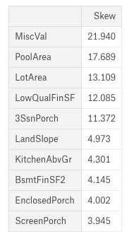
# Check the skew of all numerical features skewed_feats = all_data[numeric_feats].apply(lambda x: skew(x.dropna())).sort_values(ascending=False) print("\nSkew in numerical features: \n") skewness = pd.DataFrame({'Skew' :skewed_feats}) skewness.head(10)
Box Cox变换高斜率特征
1 2 3 4 5 6 7 8 9 10 11
skewness = skewness[abs(skewness) > 0.75] print("There are {} skewed numerical features to Box Cox transform".format(skewness.shape[0]))
from scipy.special import boxcox1p skewed_features = skewness.index lam = 0.15 for feat in skewed_features: #all_data[feat] += 1 all_data[feat] = boxcox1p(all_data[feat], lam) #all_data[skewed_features] = np.log1p(all_data[skewed_features])
train = all_data[:ntrain] test = all_data[ntrain:]
5.模型
导入相关库
1
2
3
4
5
6
7
8
9
10
from sklearn.linear_model import ElasticNet, Lasso,  BayesianRidge, LassoLarsIC
from sklearn.ensemble import RandomForestRegressor,  GradientBoostingRegressor
from sklearn.kernel_ridge import KernelRidge
from sklearn.pipeline import make_pipeline
from sklearn.preprocessing import RobustScaler
from sklearn.base import BaseEstimator, TransformerMixin, RegressorMixin, clone
from sklearn.model_selection import KFold, cross_val_score, train_test_split
from sklearn.metrics import mean_squared_error
import xgboost as xgb
import lightgbm as lgb
classAveragingModels(BaseEstimator, RegressorMixin, TransformerMixin): def__init__(self, models): self.models = models # we define clones of the original models to fit the data in deffit(self, X, y): self.models_ = [clone(x) for x in self.models] # Train cloned base models for model in self.models_: model.fit(X, y)
return self #Now we do the predictions for cloned models and average them defpredict(self, X): predictions = np.column_stack([ model.predict(X) for model in self.models_ ]) return np.mean(predictions, axis=1)
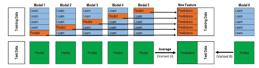
classStackingAveragedModels(BaseEstimator, RegressorMixin, TransformerMixin): def__init__(self, base_models, meta_model, n_folds=5): self.base_models = base_models self.meta_model = meta_model self.n_folds = n_folds # We again fit the data on clones of the original models deffit(self, X, y): self.base_models_ = [list() for x in self.base_models] self.meta_model_ = clone(self.meta_model) kfold = KFold(n_splits=self.n_folds, shuffle=True, random_state=156) # Train cloned base models then create out-of-fold predictions # that are needed to train the cloned meta-model out_of_fold_predictions = np.zeros((X.shape[0], len(self.base_models))) for i, model in enumerate(self.base_models): for train_index, holdout_index in kfold.split(X, y): instance = clone(model) self.base_models_[i].append(instance) instance.fit(X[train_index], y[train_index]) y_pred = instance.predict(X[holdout_index]) out_of_fold_predictions[holdout_index, i] = y_pred # Now train the cloned meta-model using the out-of-fold predictions as new feature self.meta_model_.fit(out_of_fold_predictions, y) return self #Do the predictions of all base models on the test data and use the averaged predictions as #meta-features for the final prediction which is done by the meta-model defpredict(self, X): meta_features = np.column_stack([ np.column_stack([model.predict(X) for model in base_models]).mean(axis=1) for base_models in self.base_models_ ]) return self.meta_model_.predict(meta_features)